Author: Brian Ribeiro

Understanding Torque Curves: Why They Matter When Selecting a VFD
When selecting a Variable Frequency Drive (VFD), it’s easy to focus on horsepower, voltage, or cost. But one of the most critical—and often overlooked—factors is the torque curve of the application. Understanding torque requirements ensures your VFD is properly matched to the load, delivering reliable performance, energy efficiency, and long equipment life.

What Is a Torque Curve?

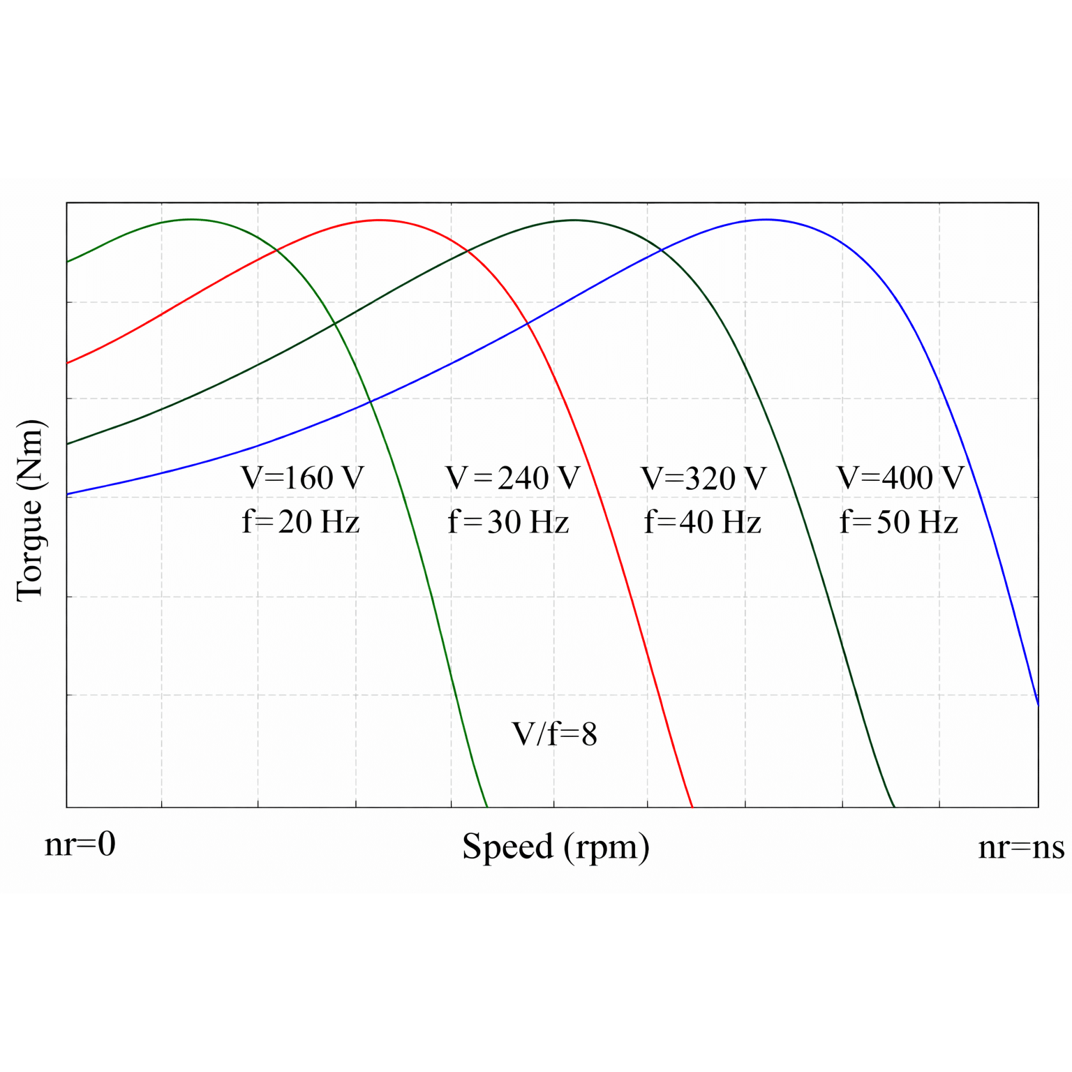
A torque curve shows how much torque (rotational force) a motor or application requires across different speeds. Every type of load—whether it’s a fan, pump, or conveyor—has its own unique torque profile.

At its core:
- Torque = the force needed to rotate a load
- Speed = how fast that load rotates
The relationship between the two determines how your system behaves—and how your VFD should be configured.

The Three Main Types of Torque Loads
1. Variable Torque Loads (Fans & Pumps)
- Torque increases with the square of speed
- Power increases with the cube of speed
Examples:
- HVAC fans
- Centrifugal pumps
Why it matters:

This is where VFDs shine. Reducing speed even slightly leads to significant energy savings. Selecting a VFD optimized for variable torque can dramatically cut operating costs.
1. Constant Torque Loads (Conveyors & Compressors)
- Torque remains constant regardless of speed
Examples:
- Conveyors
- Positive displacement pumps
- Screw compressors
Why it matters:

These applications require steady force at all speeds. Your VFD must be sized to handle full torque even at low speeds, or you risk stalling and overheating.
1. Constant Horsepower Loads (Machine Tools)
- Torque decreases as speed increases
- Horsepower remains constant
Examples:
- Machine tool spindles
- Winder/unwinder systems
Why it matters:

These applications require precise control across a wide speed range. A properly selected VFD ensures smooth transitions and consistent performance.

Why Torque Curves Matter in VFD Selection
1. Proper Sizing
Choosing a VFD without understanding torque can lead to:
- Undersized drives → stalling, trips, overheating
- Oversized drives → unnecessary cost
Matching the torque curve ensures the drive delivers the right amount of power exactly when needed.
1. Energy Efficiency
Different torque profiles respond differently to speed control:
- Variable torque loads = massive energy savings
- Constant torque loads = more stable, predictable consumption
Understanding this helps maximize ROI from your VFD investment.
1. System Reliability
If torque demands aren’t met:
- Motors can overheat
- Drives can trip
- Equipment life is reduced
A properly matched torque profile keeps everything running smoothly and extends system lifespan.
1. Control Strategy Optimization
Torque characteristics influence:
- Acceleration and deceleration settings
- Control modes (V/Hz vs vector control)
- Protection parameters
This ensures optimal performance for your specific application.

Common Mistakes to Avoid
- Assuming all loads behave the same
(Fans ≠ conveyors ≠ compressors)
- Ignoring starting torque requirements
Some applications need a torque boost at startup
- Overlooking low-speed performance
Critical for conveyors and heavy loads
- Not accounting for load variations
Real-world conditions often differ from ideal curves

Bringing It All Together

Selecting the right VFD isn’t just about matching voltage and horsepower—it’s about understanding how your system behaves under real operating conditions.

Torque curves provide that insight.

By aligning your VFD selection with your application’s torque profile, you can:
- Improve efficiency
- Enhance reliability
- Reduce operating costs
- Extend equipment life
Final Thought

In today’s push for smarter, more energy-efficient systems, torque curves are more than just engineering theory—they’re a practical tool for better decision-making.

Get the torque right, and everything else follows.
April 9, 2026
Understanding UPS Harmonic Mitigation and THDi/THDv
Uninterruptible Power Supply (UPS) systems are essential for protecting critical loads—from data centers and healthcare facilities to industrial automation and control systems. But beyond backup power, UPS systems can also play a key role in power quality, particularly when it comes to harmonics.

Understanding how UPS systems interact with harmonics—and how to evaluate THDi (Total Harmonic Distortion of Current) and THDv (Total Harmonic Distortion of Voltage)—is critical for designing reliable, efficient electrical systems.

What Are Harmonics?

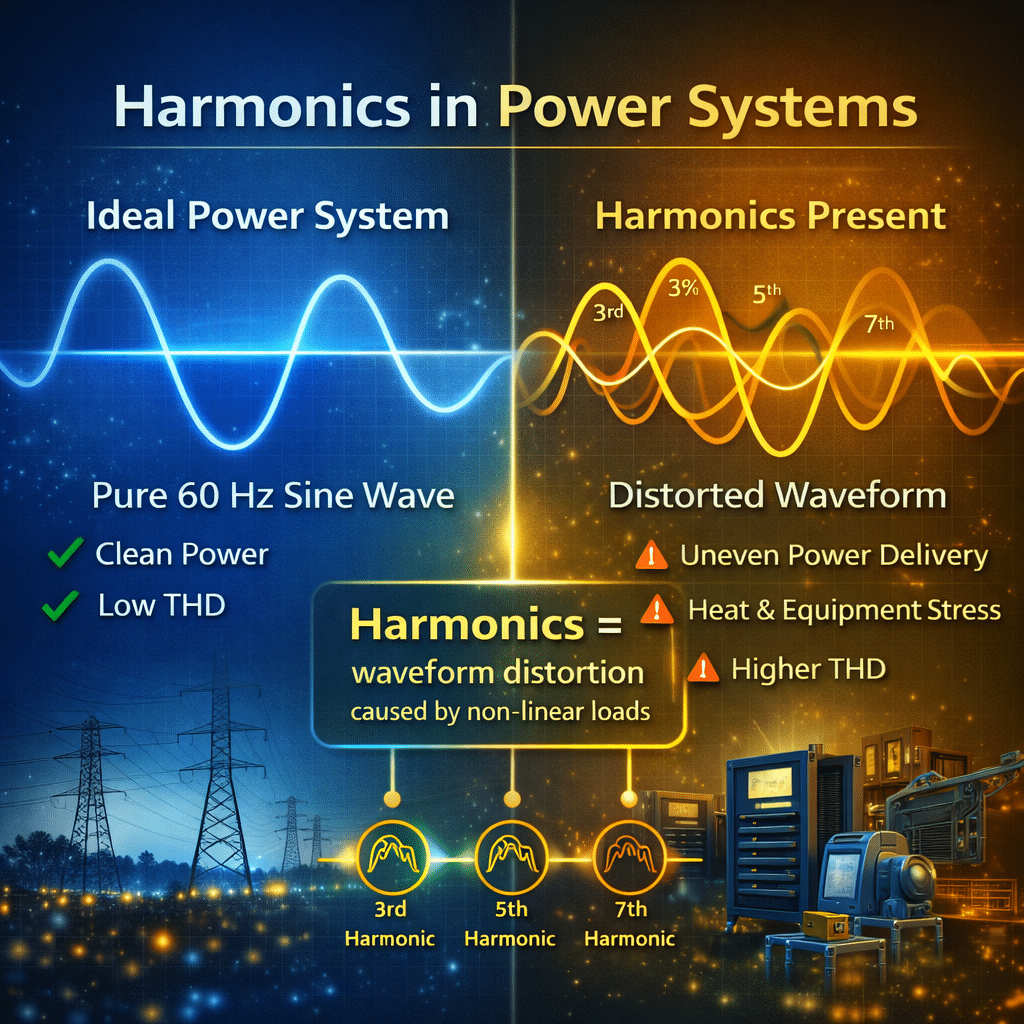
Harmonics are distortions in electrical waveforms caused by non-linear loads. Instead of a smooth sine wave, the current or voltage waveform becomes distorted.

Common sources include:
- Variable Frequency Drives (VFDs)
- Switch-mode power supplies
- LED lighting
- UPS systems themselves
These distortions can lead to:
- Overheating of equipment
- Increased losses
- Nuisance tripping
- Reduced equipment lifespan
Visualizing Harmonics

A pure sine wave represents ideal power. Harmonics introduce additional frequencies (multiples of the fundamental frequency), distorting the waveform.

What Is THDi vs. THDv?

THDi (Total Harmonic Distortion – Current)
- Measures distortion in current waveform
- Expressed as a percentage of the fundamental current
Indicates how much harmonic current a device injects into the system

THDv (Total Harmonic Distortion – Voltage)
- Measures distortion in voltage waveform
- Expressed as a percentage of the fundamental voltage
Reflects the impact of harmonic currents on system voltage

Key Relationship
- Non-linear loads → create harmonic currents (THDi)
- System impedance → converts THDi into voltage distortion (THDv)
High THDi can lead to high THDv, depending on the system.

Why Harmonics Matter in UPS Systems

UPS systems can both:
- Generate harmonics (especially older or less advanced designs)
- Mitigate harmonics (with modern technologies)
Risks of Poor Harmonic Performance
- Overheating of transformers and cables
- Reduced generator compatibility
- Interference with sensitive equipment
- Lower overall system efficiency
Modern UPS Harmonic Mitigation Techniques
1. Active Front End (AFE) Rectifiers
- Uses IGBT-based converters
- Draws near-sinusoidal input current
- Achieves very low THDi (often < 3%)
One of the most effective harmonic mitigation solutions
1. Passive Harmonic Filters
- Uses inductors and capacitors
- Reduces harmonic distortion at specific frequencies
Pros:
- Cost-effective
- Simple design
Cons:
- Less flexible
- Larger footprint
1. Multi-Pulse Rectifiers (12-pulse, 18-pulse)
- Uses phase-shifting transformers
- Cancels out certain harmonic components
Typical performance:
- 12-pulse: ~10–12% THDi
- 18-pulse: ~5–8% THDi
1. Active Harmonic Filters (External)
- Dynamically injects counter-harmonics
- Can be used system-wide (not just UPS)
Typical THDi and THDv Targets

Parameter

Recommended Range

THDi (UPS input)

< 5% (modern systems)

THDv (system voltage)

< 5% (per IEEE 519 guidelines)

Staying within these limits ensures:
- Compliance with standards
- Reliable system operation
- Protection of connected equipment
Real-World Impact
1. Generator Compatibility
High THDi can cause:
- Generator overheating
- Voltage instability
- Poor performance
Low-THDi UPS systems improve generator sizing and stability.
1. Energy Efficiency
Harmonics increase:
- Resistive losses
- Heat generation
Reducing harmonics improves:
- Overall system efficiency
- Operating costs
1. Equipment Lifespan
Lower harmonic distortion:
- Reduces thermal stress
- Minimizes insulation damage
- Extends equipment life
1. System Reliability
Clean power ensures:
- Stable operation of sensitive electronics
- Fewer unexpected failures
- Reduced downtime
Common Mistakes to Avoid
- Focusing only on THDv and ignoring THDi
(Both are important and interconnected)
- Assuming all UPS systems have low harmonics
(Older designs can have high THDi)
- Ignoring upstream/downstream impacts
(Harmonics affect the entire system)
- Not considering generator interaction
(Critical for backup systems)

How to Choose the Right UPS for Harmonic Performance

Ask these key questions:
1. What is the UPS input THDi rating?
2. Does it use an AFE rectifier or multi-pulse design?
3. Will it operate with a generator?
4. What are the system THDv requirements?
5. Is additional filtering needed?
Bringing It All Together

Harmonics are a critical—but often underestimated—aspect of UPS system design.
- THDi tells you how much distortion your UPS introduces
- THDv tells you how that distortion affects your system
Modern UPS technologies, especially those with active front ends, can significantly reduce harmonic impact—improving efficiency, reliability, and compliance.

Final Thought

In today’s power-sensitive environments, it’s not just about keeping the lights on—it’s about keeping the power clean.

Understanding and managing harmonics ensures your UPS system not only protects your load—but enhances the entire electrical system.
April 9, 2026
The Importance of Power Factor in Data Center UPS Selection
When selecting a UPS for a data center, power factor (PF) is one of the most misunderstood—and most costly—parameters to overlook. Two UPS systems with the same kVA rating can support very different real loads depending on their power factor. In modern, high-density data centers, that difference directly affects capacity, efficiency, scalability, and total cost of ownership.

Let’s break down why power factor matters, how it impacts UPS sizing, and what to look for in modern UPS designs.

What Is Power Factor (and Why It Matters)?

Power factor describes how effectively electrical power is converted into useful work.

Power Factor = kW (Real Power) / kVA (Apparent Power)
- kW (Real Power): Does the actual work (servers, storage, networking)
- kVA (Apparent Power): What the UPS and electrical infrastructure must deliver
- kVAR (Reactive Power): Circulating energy that does no useful work
A lower power factor means more current is required to deliver the same real power—placing greater stress on the UPS, cabling, and upstream distribution.

Why Data Centers Are Especially Sensitive to Power Factor

Modern data centers differ from traditional industrial loads in key ways:
- Server power supplies are nonlinear loads
- High rack densities drive current up quickly
- UPS systems are often sized close to limits
- Expansion happens faster than expected
A small mismatch between kVA and kW capability can strand capacity—or force an expensive upgrade far sooner than planned.

The kVA vs. kW Trap in UPS Selection

Historically, many UPS systems were rated at 0.8 power factor.

Example: Legacy UPS
- 100 kVA UPS
- PF = 0.8
- Usable real power = 80 kW
That means 20% of the UPS capacity is unusable for real IT load.

Modern UPS (Unity Power Factor)
- 100 kVA UPS
- PF = 1.0
- Usable real power = 100 kW
Same footprint. Same kVA. 25% more usable capacity.

Why Unity Power Factor UPS Systems Matter
1. Maximizes Usable Capacity
With PF ≈ 1.0:
- kW ≈ kVA
- No stranded capacity
- Better utilization of electrical infrastructure
This is especially critical in colocation and hyperscale environments where power is monetized per kW.
1. Better Match for Modern IT Loads
Most modern server power supplies:
- Use active PFC
- Draw current close to unity PF
- Expect the UPS to deliver real power, not just apparent power
A UPS with a low PF rating becomes the bottleneck—even if servers are efficient.
1. Improved Energy Efficiency
Lower power factor increases:
- RMS current
- I²R losses in cables and transformers
- Heat in switchgear and UPS components
Higher PF UPS systems:
- Reduce internal losses
- Improve overall data center PUE
- Lower cooling demand
1. Simplifies Growth and Capacity Planning
With unity PF:
- 1 kVA ≈ 1 kW
- Fewer conversion assumptions
- Cleaner planning models for expansion
This matters when scaling from:
- 500 kW → 1 MW
- Single room → multi-hall facilities
Input Power Factor vs. Output Power Factor

UPS systems have two PF considerations:

Input power factor
- How the UPS draws power from the utility
- Modern rectifiers often achieve ≥0.99
- Reduces upstream transformer and generator sizing
Output power factor
- How much real power the UPS can deliver to loads
- This is the critical spec for IT capacity
- Should be close to unity for modern data centers
Both matter—but output PF determines usable load capacity.

Impact on Generators and Electrical Infrastructure

Lower PF means:
- Higher current
- Larger generators
- Larger breakers and cabling
- Increased fault currents
A unity PF UPS:
- Reduces generator oversizing
- Improves generator-UPS compatibility
- Simplifies coordination and protection
Battery Runtime and Power Factor

Battery systems are rated in kW, not kVA.

If a UPS is kVA-limited:
- Batteries may be capable of more real power than the UPS can deliver
- Runtime calculations become misleading
Unity PF ensures:
- Battery capacity aligns with usable UPS output
- Runtime specs match real-world performance
Key Questions to Ask When Selecting a UPS
1. What is the output power factor at full load?
2. Is the UPS kVA-limited or kW-limited?
3. How does PF affect future rack density?
4. Does the UPS align with modern server PFC behavior?
5. How does PF impact generator sizing and fuel efficiency?
Common Mistakes in UPS Power Factor Selection
- Assuming all 100 kVA UPS systems deliver 100 kW
- Ignoring output PF while focusing only on efficiency
- Oversizing UPS capacity to compensate for low PF
- Discovering stranded capacity during expansion
These mistakes are expensive—and entirely avoidable.

The Bottom Line

In data centers, power factor is not a secondary spec—it’s a capacity spec.

Choosing a UPS with high or unity output power factor:
- Maximizes usable IT load
- Improves efficiency and PUE
- Reduces infrastructure costs
- Future-proofs growth
When evaluating UPS systems, always ask:

How much real power can this UPS actually deliver?
March 4, 2026

Parameter	Recommended Range
THDi (UPS input)	< 5% (modern systems)
THDv (system voltage)	< 5% (per IEEE 519 guidelines)

How Gate Charge Impacts Switching Performance in MOSFETs and IGBTs

When engineers evaluate power semiconductors, they often focus on voltage rating, current rating, and conduction losses. But in real switching applications—especially at high frequency—gate charge plays a major role in determining efficiency, switching speed, EMI, and even device reliability.

Understanding how gate charge affects MOSFETs and IGBTs helps you select the right device and the right gate driver for your application.

What Is Gate Charge?

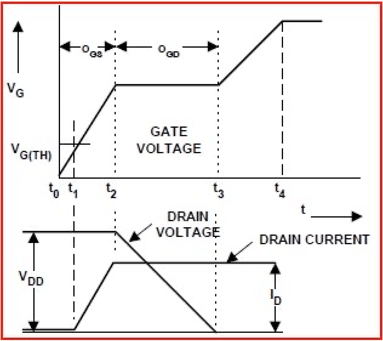
Gate charge (Qg) is the total amount of electrical charge required to drive a power device from OFF to ON at a specified gate voltage.

It is not a single number—it’s the sum of several components:

Qgs – charge to raise the gate-to-source/emitter voltage to the threshold
Qgd (Miller charge) – charge required during the drain/collector voltage transition
Qg(total) – total charge needed for full enhancement

Gate charge directly determines how fast a device can switch for a given gate driver strength.

Why Gate Charge Matters

The gate is capacitive. To switch the device, the driver must move charge in and out of the gate.

This affects:

Switching speed
Switching losses
Driver power requirements
EMI and dv/dt behavior
Maximum practical switching frequency

Key relationship

Switching speed ∝ Gate driver current / Gate charge

Gate Charge and Switching Losses

During switching transitions:

Voltage across the device is high
Current through the device is high

This overlap causes switching losses, which increase as switching slows down.

Higher gate charge → slower transitions → higher switching losses.

MOSFETs: Gate Charge Behavior

Characteristics

Voltage-controlled device
No minority carrier storage
Very fast switching capability

Gate charge implications

Qg scales strongly with die size
Low-Rds(on) MOSFETs often have high Qg
Miller plateau (Qgd) dominates high-voltage switching

Practical impact

Low Qg → high-frequency capability (100 kHz+)
High Qg → requires strong gate drivers
Gate charge often limits efficiency before conduction losses do

Design tradeoff

Lower Rds(on) ≠ better overall efficiency if Qg is too high for the switching frequency

IGBTs: Gate Charge Behavior

Characteristics

MOS gate with bipolar conduction
Minority carrier device
Lower conduction loss at high voltage

Gate charge implications

Total Qg is often lower than large MOSFETs
Switching is limited more by carrier tail current than Qg
Turn-off losses dominate at high frequency

Practical impact

Well suited for low–to–medium switching frequencies
Gate charge still affects dv/dt and EMI
Faster gate drive can reduce switching loss—but only to a point

Key limitation

Even with low gate charge, stored charge in the drift region limits IGBT switching speed

Miller Charge: The Real Bottleneck

The Miller charge (Qgd) occurs while:

Gate voltage is “stuck” at the Miller plateau
Drain/collector voltage is actively changing

During this time:

Gate current controls dv/dt
EMI and overshoot are set
Switching loss accumulates

Devices with lower Qgd:

Switch faster
Produce less switching loss
Are easier to control cleanly

Gate Charge vs. Gate Driver Design

Gate charge must always be considered together with the gate driver.

Gate driver current

t_sw Q_g / I_gate

High Qg → needs high peak gate current
Weak drivers → slow switching → excess loss
Strong drivers → faster switching but higher EMI risk

This is why gate resistors, split turn-on/turn-off resistors, and active gate control are so common.

MOSFET vs. IGBT: Gate Charge Comparison

Parameter	MOSFET	IGBT
Gate type	Capacitive	Capacitive
Total gate charge	Often higher	Often lower
Miller dominance	Very high	Moderate
Switching frequency	Very high	Moderate
Limiting factor	Qg + Qgd	Tail current
Best use case	High-frequency	High-voltage, lower-frequency

Practical Design Guidelines

Compare Qg and Qgd, not just Rds(on) or Vce(sat)
Match gate driver peak current to total gate charge
Don’t overspeed switching without managing EMI
For high frequency → prioritize low Qgd MOSFETs
For high voltage & power → accept slower switching IGBTs
Validate with real waveforms—not just datasheets

The Bottom Line

Gate charge is one of the most important—and most misunderstood—parameters in power semiconductor selection.

MOSFETs are often limited by gate charge at high frequency
IGBTs are limited more by stored charge, but gate charge still shapes switching behavior
Gate charge directly links device physics to real-world efficiency

Designing efficient, reliable power electronics means treating the device and gate driver as a system, not separate components.

March 4, 2026

How Pressure, Vacuum, and Airflow Interact in Regenerative Blower Systems
Regenerative blowers are deceptively simple machines. With no internal contact and a single rotating impeller, they generate both pressure and vacuum—but understanding how those forces interact with airflow is the key to sizing, efficiency, and reliability.

If pressure, vacuum, and airflow aren’t properly matched to the application, even a high-quality blower can underperform or fail prematurely. Let’s break down how these three variables work together.

The Basics: One Blower, Two Modes

A regenerative blower operates on the same aerodynamic principle whether it’s producing pressure or vacuum:
- Pressure mode → air is pushed into the system
- Vacuum mode → air is pulled from the system
The blower itself doesn’t change—only how the inlet and outlet are connected.

Airflow: The Foundation Variable

Airflow (usually measured in CFM or m³/h) is the starting point for understanding blower behavior.

Key truth

A regenerative blower does not create pressure first—it creates airflow first.

As airflow encounters resistance in the system, pressure or vacuum develops.

Pressure and Vacuum: Resistance to Airflow

Pressure and vacuum are simply two sides of the same coin:
- Pressure = resistance on the discharge side
- Vacuum = resistance on the inlet side
Both are caused by system restrictions such as:
- Pipe length and diameter
- Filters and silencers
- Diffusers, air knives, manifolds
- Process backpressure
The Blower Curve: Where Everything Connects

Every regenerative blower has a performance curve that shows the relationship between:
- Airflow (horizontal axis)
- Pressure or vacuum (vertical axis)
What the curve tells you
- Maximum airflow occurs at near-zero pressure
- Maximum pressure or vacuum occurs at near-zero airflow
- Normal operation happens somewhere in between
Your system determines where on that curve the blower operates.

Pressure vs. Airflow Trade-Off

As system resistance increases:
- Airflow decreases
- Pressure or vacuum increases
This trade-off is unavoidable and fundamental to regenerative blower operation.

Common misconception

“I need high airflow and high pressure.”

In reality, the system can only get one at the expense of the other unless the blower size or speed changes.

System Curve: The Missing Half of the Equation

Your piping and process create a system curve—a graphical representation of how much pressure or vacuum is required at different airflow rates.
- Long piping → steeper curve
- Dirty filters → curve shifts upward
- Valves closing → curve steepens instantly
The actual operating point is where the blower curve intersects the system curve.

Pressure Mode vs. Vacuum Mode: Subtle Differences

While the physics are the same, practical differences matter:

Pressure mode
- Heat builds up on the discharge side
- Overpressure can overload the motor
- Relief valves are often critical
Vacuum mode
- Inlet filters play a major role
- Clogging increases vacuum rapidly
- Risk of overheating at low airflow
Heat: The Silent Fourth Variable

As pressure or vacuum increases and airflow decreases:
- Less air moves through the blower for cooling
- Internal temperature rises
This is why deadheading (near-zero airflow) is dangerous—even if pressure limits aren’t exceeded.

Why Oversizing Isn’t a Fix

A larger blower:
- May push the operating point into inefficient regions
- Can increase noise and energy consumption
- Doesn’t eliminate system restrictions
Correct sizing means:
- Matching airflow requirements
- Accounting for worst-case pressure or vacuum
- Staying within the blower’s efficient operating range
Practical Design Tips
- Size blowers using both airflow and pressure/vacuum
- Account for dirty filters and future expansion
- Avoid operating near maximum pressure or vacuum continuously
- Use relief valves or bypasses when airflow can be restricted
- Verify cooling at low-flow conditions
The Bottom Line

In regenerative blower systems:
- Airflow creates pressure and vacuum
- System resistance determines how much of each you get
- The blower curve and system curve define real performance
Understanding how pressure, vacuum, and airflow interact helps you select the right blower, prevent overheating, and achieve stable, efficient operation across the full life of the system.
March 4, 2026
Why Sensor Drift Happens—and How Modern Pressure Transmitters Compensate for It
Pressure transmitters are expected to deliver reliable, accurate measurements year after year—even in harsh industrial environments. Yet over time, many instruments slowly deviate from their original calibration. This phenomenon, known as sensor drift, is unavoidable to some degree—but modern pressure transmitters are far better at detecting, correcting, and compensating for it than earlier generations.

Understanding why drift occurs—and how today’s transmitters fight it—can help reduce maintenance costs, prevent bad process decisions, and improve long-term system reliability.

What Is Sensor Drift?

Sensor drift is a gradual change in a pressure transmitter’s output that is not caused by an actual change in process pressure. It typically shows up as:
- Zero drift – output shifts when pressure is at zero
- Span drift – gain changes across the measurement range
- Non-linear drift – distortion at specific pressure points
Unlike sudden failure, drift is subtle—and dangerous precisely because it often goes unnoticed.

Why Sensor Drift Happens
1. Mechanical Stress and Material Fatigue
Pressure sensors rely on diaphragms or sensing elements that flex under load. Repeated pressure cycling—especially near the upper range—causes microscopic mechanical changes over time.

Common contributors
- High cycle counts
- Pressure spikes or pulsation
- Operation near maximum rated pressure
1. Temperature Effects
Temperature is one of the largest drivers of drift.
- Sensor materials expand and contract
- Electronics change characteristics with heat
- Outdoor or process-adjacent installations see wide swings
Without compensation, even a stable pressure can appear to “move” as ambient or process temperature changes.
1. Aging of Electronic Components
Resistors, amplifiers, and reference elements naturally drift as they age. This is especially true in older analog designs with limited self-correction capability.
1. Process and Environmental Exposure
Harsh environments accelerate drift:
- Corrosive or dirty process media
- Moisture ingress
- Vibration and mechanical shock
- EMI and electrical noise
Even a well-designed sensor will drift faster if its environment is hostile.
1. Installation and Mounting Stress
Improper mounting can introduce mechanical strain into the sensor body, subtly biasing the measurement.

Examples include:
- Over-tightened fittings
- Misaligned impulse lines
- Pipe stress transferred into the transmitter housing
How Modern Pressure Transmitters Compensate for Drift

The good news: modern pressure transmitters are designed with drift in mind—and actively work to minimize its impact.
1. Digital Temperature Compensation
Modern transmitters use embedded microprocessors to apply real-time temperature correction.

How it works
- Factory calibration across multiple temperature points
- Internal temperature sensors track real conditions
- Algorithms dynamically adjust the pressure signal
This dramatically reduces both zero and span drift caused by temperature variation.
1. Advanced Sensor Materials and Construction
Newer sensing elements are built from materials with:
- Lower hysteresis
- Improved elastic stability
- Better resistance to fatigue
Techniques such as laser-welded diaphragms and monolithic sensor designs reduce long-term mechanical drift.
1. Digital Signal Processing (DSP)
Instead of raw analog outputs, modern transmitters digitize the sensor signal early and apply filtering and correction digitally.

Benefits
- Reduced noise and EMI sensitivity
- Stable long-term gain characteristics
- Improved repeatability over time
1. Auto-Zero and Self-Diagnostics
Many smart transmitters continuously monitor their own behavior.

They can:
- Detect abnormal offset changes
- Flag drift beyond acceptable limits
- Alert operators before accuracy degrades significantly
Some systems even support in-situ zero trimming without removing the transmitter from service.
1. Long-Term Stability Specifications
Modern datasheets increasingly focus on long-term stability (e.g., ±0.1% URL over 5 or 10 years) rather than just initial accuracy.

This reflects real-world performance—not just lab conditions on day one.

Drift vs. Accuracy: A Common Misconception

A transmitter can be highly accurate when calibrated but still drift significantly over time. The most valuable instruments combine:
- High initial accuracy
- Excellent long-term stability
- Robust compensation algorithms
It’s stability—not just accuracy—that determines recalibration intervals and lifecycle cost.

Practical Ways to Minimize Drift in the Field
- Select transmitters with strong long-term stability specs
- Avoid operating continuously at maximum pressure
- Install with proper mechanical support and alignment
- Protect transmitters from extreme temperature swings
- Leverage diagnostics and calibration alerts
The Bottom Line

Sensor drift is inevitable—but unmanaged drift is optional.

Modern pressure transmitters use digital compensation, smarter electronics, and improved materials to dramatically reduce drift and extend calibration intervals. The result is more reliable data, fewer maintenance interventions, and better process control over the life of the instrument.
March 4, 2026
Understanding Tags, Data Mapping, and Variables in HMI Design
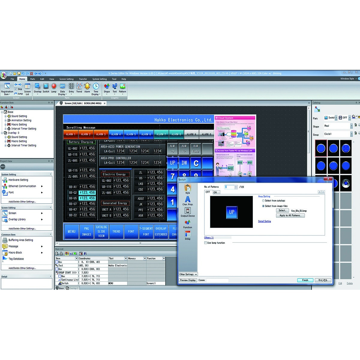
A well-designed HMI doesn’t just look good—it communicates clearly, responds instantly, and reflects what’s really happening in the process. At the heart of all of that are tags, data mapping, and variables.

These three concepts form the data backbone of any HMI system. When they’re designed thoughtfully, your HMI is fast, reliable, and easy to maintain. When they’re not, you get sluggish screens, broken animations, and operators who don’t trust what they’re seeing.

Let’s break them down.

What Is a Tag in an HMI?

A tag is a named reference to a piece of data that the HMI reads from or writes to a controller, device, or internal memory location.

Think of a tag as:

A label that connects the HMI to a real-world value

Common tag types
- Motor status (Run / Stop)
- Pressure, temperature, flow values
- Setpoints
- Alarms and fault codes
- Operator commands (Start, Reset, Acknowledge)
A good tag name is descriptive, consistent, and readable—because humans will maintain this system long after it’s deployed.

Variables vs. Tags: What’s the Difference?

This is where many new HMI designers get tripped up.

Tags
- Linked to external data sources
- Represent real process values
- Update through communications (Ethernet/IP, Modbus, PROFINET, etc.)
Variables
- Exist inside the HMI only
- Used for logic, math, animation, or temporary values
- Not directly tied to a PLC unless you map them
When to use variables
- Screen navigation logic
- Animation scaling
- Runtime calculations (averages, conversions)
- User interface state tracking
Rule of thumb:

If the value must survive a power cycle or affect the process, it belongs in the PLC (tag).

If it’s purely visual or temporary, keep it in the HMI (variable).

What Is Data Mapping?

Data mapping is the process of linking an HMI tag to its actual data source.

That source could be:
- A PLC register
- A drive parameter
- An I/O point
- Another controller
- An internal HMI variable
If the mapping is wrong—even by one address—the HMI may:
- Display incorrect values
- Fail to update
- Write data to the wrong device (worst case)
One-to-One vs. Indirect Mapping

One-to-one mapping
- Each tag maps directly to one PLC address
- Simple, clear, easy to troubleshoot
- Preferred for most systems
Indirect (indexed) mapping
- Tag address changes dynamically using an index or pointer
- Reduces tag count
- Increases complexity and risk
Indirect mapping is powerful—but best reserved for advanced applications with strong documentation.

Why Good Tag Design Matters

Poor tag design leads to:
- Slow screen refresh
- Communication overload
- Difficult troubleshooting
- Risky future expansions
Good tag design enables:
- Faster development
- Easier maintenance
- Better alarm handling
- Cleaner screen logic
Best Practices for HMI Tags and Variables
1. Use Consistent Naming Conventions
2. Avoid Duplicating Logic
- Don’t recreate PLC logic in the HMI
- Let the PLC control the process
- Let the HMI visualize and command
1. Limit High-Speed Polling
- Only update fast-changing tags when needed
- Group tags by update rate (fast, normal, slow)
1. Separate Process Data from UI Logic
- Process values → PLC tags
- Screen states, animations → HMI variables
1. Document Everything
Good documentation beats clever shortcuts every time.

Tags, Alarms, and Performance

Every tag consumes:
- Network bandwidth
- PLC scan time
- HMI processing power
Well-structured tag databases:
- Reduce network traffic
- Improve alarm response
- Keep screens responsive
This becomes critical in systems with:
- Hundreds of alarms
- Multiple HMIs
- Remote connections
Common HMI Data Design Mistakes
- Using the HMI as a “soft PLC”
- Poor or cryptic tag names
- Mapping unused tags
- Mixing UI logic and process control
- Ignoring update rates
These issues don’t always show up during commissioning—but they surface later during troubleshooting or expansion.

The Bottom Line

In HMI design:
- Tags connect your screens to the real world
- Data mapping ensures those connections are accurate
- Variables handle internal logic and visualization
Mastering these fundamentals leads to HMIs that are faster, clearer, and far easier to maintain—long after the original designer has moved on.
March 4, 2026
How to Properly Size a Contactor for Inductive vs. Resistive Loads
Sizing a contactor isn’t just “match the amps.” Inductive loads (motors, transformers, solenoids) create inrush current and switching transients that are much harder on contacts than resistive loads (heaters, incandescent lamps). The right way to size a contactor is to size to the utilization category / duty and the real switching conditions, not just steady-state current.

Step 1: Identify the load type and what you’re switching

Resistive loads (easy on contacts)

Examples: electric heaters, ovens, radiant elements
- Current is close to steady-state immediately
- Power factor ~1
- Minimal inrush (except some lamps)
Inductive loads (hard on contacts)

Examples: motors, compressors, transformers, solenoids
- High inrush / locked-rotor current
- Lower power factor
- Arcing is worse at opening; contact wear increases
Also note how you’re switching:
- Making current (closing) can cause weld risk under high inrush
- Breaking current (opening) can cause heavy arcing under inductive loads
- Jogging/inching (rapid cycling) is especially abusive
Step 2: Use the correct utilization category (IEC) or duty rating (NEMA)

This is the single biggest “do it right” factor.

IEC (common in modern spec sheets)
- AC-1: non-inductive / slightly inductive (resistive heating)
- AC-3: squirrel-cage motor starting + stopping while running (typical motor duty)
- AC-4: inching/jogging, plugging (very severe motor duty)
Rule of thumb:

A contactor that’s “40 A AC-1” might be only “18–25 A AC-3” for motor duty at the same voltage.

NEMA (common in North America)

NEMA sizes (00, 0, 1, 2, 3…) bundle conservative motor-duty assumptions. If you specify by NEMA size, you’re largely specifying for inductive motor service.

Step 3: Calculate the current you should size to
1. A) Resistive load sizing (AC-1)
1. Find heater current:
I = P / V (single-phase)

I = P / V (3-phase)
1. Apply margin for continuous duty and enclosure temperature:
- Typical: 1.25× for continuous heating loads (and/or per code/internal standard)
- Add more margin if ambient is hot, panel is crowded, or switching is frequent
Practical target: pick a contactor with AC-1 rating ≥ 125% of steady current.

Example: 12 kW heater @ 240 V 1φ
- I = 12,000 / 240 = 50 A
- 125% → 62.5 A → choose ~65 A AC-1 contactor
1. B) Inductive load sizing (motor / AC-3, AC-4)
For motors, start with motor FLA (from the nameplate). Then size by duty category and starting method:

1) Standard motor start/stop (AC-3)
- Choose contactor with AC-3 current rating ≥ motor FLA at the motor voltage
- If high cycling, high ambient, or poor power factor → add margin
2) Inching/jogging or plugging (AC-4)
- Don’t “add a little margin”—you often need a much larger contactor, or a different control approach
- AC-4 ratings are significantly lower than AC-3 at the same frame size
3) High inrush loads
- Motors: inrush can be 5–8× FLA (or higher) at start
- Solenoids/transformers: inrush can be 10–15× momentarily
A properly rated motor-duty contactor is designed to tolerate this—if you selected the correct AC category.

Example: 15 HP, 460 V, 3φ motor (nameplate FLA ~ 21 A-ish; use actual nameplate)
- Select contactor where AC-3 ≥ 21 A at 460 V
- If jogging/inching → choose based on AC-4 (likely a larger frame)
Step 4: Confirm the “hidden” specs that cause failures

Electrical life vs mechanical life
- Resistive loads typically allow longer electrical life
- Inductive loads shorten electrical life drastically
Check switching frequency and required service life.

Coil voltage and control scheme
- Correct coil voltage (120 VAC, 24 VDC, etc.)
- For DC coils: ensure proper suppression (or use built-in) to protect PLC outputs
Short-circuit protection and coordination

A contactor’s survival in a fault depends on upstream protection and coordination:
- Verify SCCR (short-circuit current rating) for the assembly
- Check manufacturer coordination tables (contactor + fuse/breaker)
Ambient temperature and enclosure

Heat derates contactors. If your panel runs hot, upsize or provide ventilation.

Quick “cheat sheet”

Resistive (heaters, AC-1):
- Size to steady current × 1.25
- Watch ambient heat and cycling rate
Inductive (motors, AC-3):
- Size to motor FLA at voltage using AC-3 rating
- Add margin for frequent starts/thermal environment
Severe motor duty (AC-4):
- Expect to upsize significantly
- Consider soft starters/VFDs to reduce abuse
Most common sizing mistakes
- Using AC-1 amps for motor duty
- Ignoring AC-4 when there’s jogging/inching
- Not checking SCCR/coordination with the protective device
- Forgetting temperature derating in a hot enclosure
March 4, 2026
How to Match an AC Drive to Different Motor Types
Selecting the right AC drive isn’t just about horsepower and voltage. The motor type you’re controlling—induction, permanent magnet (PM), or synchronous reluctance (SynRM)—has a major impact on drive sizing, control method, efficiency, and long-term performance. Match them correctly, and you get smooth control, high efficiency, and long motor life. Get it wrong, and you invite instability, overheating, or lost efficiency.

Below is a practical breakdown of what to consider for each motor type.
1. Induction Motors (IM)
Why they’re common

Induction motors are the workhorse of industry—rugged, affordable, and widely available. Most legacy systems were built around them.

Drive considerations

Control method
- V/Hz (scalar control):
  - Simple, low cost
  - Best for pumps, fans, conveyors
  - Limited torque control at low speeds
- Sensorless vector or closed-loop vector:
  - Better torque and speed accuracy
  - Recommended for demanding loads
Sizing
- Match drive current rating to motor FLA, not just HP
- Account for overload requirements (typically 150% for 60 seconds)
Key parameters
- Motor rated voltage, current, frequency, speed
- Slip compensation (important for torque accuracy)
Best-fit applications
- Fans, pumps, compressors
- General-purpose machinery
- Retrofit projects
1. Permanent Magnet Motors (PM / PMSM / BLDC)
Why they’re growing fast

PM motors offer higher efficiency, higher power density, and better part-load performance—making them ideal for energy-savings programs and premium OEM designs.

Drive considerations

Drive compatibility
- The drive must explicitly support PM motors
- Requires vector control or FOC (Field-Oriented Control)
Critical differences
- No rotor losses → higher efficiency
- Magnets create back EMF → overspeed protection is essential
- Incorrect setup can cause uncontrolled voltage rise
Key parameters
- Motor back-EMF constant (Ke)
- Pole count
- Rated speed and max mechanical speed
- Encoder feedback (optional but helpful for precision)
Best-fit applications
- HVAC (chillers, compressors)
- High-efficiency pumps and fans
- EVs and high-performance machinery
1. Synchronous Reluctance Motors (SynRM)
Why they’re gaining attention

SynRM motors deliver high efficiency without rare-earth magnets, making them attractive where sustainability, cost stability, and reliability matter.

Drive considerations

Control method
- Requires advanced vector control
- Many modern drives support SynRM with firmware configuration
Performance traits
- High efficiency similar to PM motors
- No magnets → simpler thermal behavior
- Torque ripple can occur if control tuning is poor
Key parameters
- d-axis and q-axis inductances
- Motor identification routine (often required at startup)
- Proper torque model selection in the drive
Best-fit applications
- Energy-efficient pump and fan systems
- Industrial processes seeking PM-like efficiency
- Sites avoiding rare-earth materials
Practical Selection Tips
- Confirm motor compatibility first – not all drives support PM or SynRM motors
- Size by current, not HP alone – especially for PM motors
- Use motor auto-tuning whenever available
- Check overspeed and braking requirements for PM motors
- Align drive features with incentives if energy efficiency matters
Bottom line

An AC drive isn’t one-size-fits-all. Induction motors favor simplicity, PM motors reward precision, and SynRM motors strike a balance between efficiency and material sustainability. Matching the drive correctly unlocks the full potential of each motor type—whether your goal is reliability, efficiency, or performance.
March 4, 2026

UPS Systems and Regulatory Compliance: NFPA, Uptime Institute, and More

UPS (Uninterruptible Power Supply) systems are not just about keeping the lights on—they are a critical part of regulatory compliance in data centers, healthcare, finance, manufacturing, and other mission-critical industries. Whether you’re protecting sensitive data or life-safety systems, your UPS system must align with industry codes and standardsto ensure safety, reliability, and legal compliance.

Why Regulatory Compliance Matters

Safety: Prevent injury or equipment failure in critical environments.
Reliability: Meet service-level agreements (SLAs) and uptime targets.
Audit Readiness: Avoid penalties and ensure certifications remain valid.
Insurance & Liability: Compliance can reduce exposure to claims or denied coverage.

NFPA (National Fire Protection Association)

NFPA 70 – National Electrical Code (NEC)

Article 701/700/702: Covers emergency, legally required, and optional standby systems.
UPS systems must be properly classified and installed according to their role (e.g., life safety vs. IT loads).

NFPA 111 – Stored Electrical Energy Emergency and Standby Power Systems

Directly applies to UPS systems.
Covers:
- Installation, performance, and testing requirements
- Battery storage, ventilation, and monitoring
- Maintenance intervals and test procedures
Required for life safety and critical operation power systems (COPS)

Uptime Institute Tier Standards

Tier I–IV Certification Criteria

UPS systems are essential to achieving Tier III and IV ratings, which require:
- Redundancy (e.g., N+1, 2N)
- Concurrent maintainability (Tier III)
- Fault tolerance (Tier IV)
UPS design must support continuous availability with no single point of failure.
Modular, scalable UPS systems help meet Tier goals more efficiently.

Healthcare Facility Standards

NFPA 99 – Health Care Facilities Code

UPS systems may be required for critical care areas to ensure power to life-support equipment.
Must be compliant with Type 1 Essential Electrical Systems.
Requires battery backup with transfer times compliant with code (<10 seconds for critical systems).

Other Relevant Standards and Guidelines

Standard	Area of Relevance
IEC 62040	Global UPS design and safety standard
UL 1778	UPS safety compliance (North America)
OSHA 1910 Subpart S	General electrical safety, includes backup power systems
ISO/IEC 27001	Data protection and business continuity (recommends UPS for risk mitigation)
TAA, RoHS, ENERGY STAR	Environmental and procurement compliance for federal/government clients

Best Practices for Compliance

Document everything: Maintenance logs, test results, commissioning reports
Perform regular testing: Including battery discharge, bypass verification, and load testing
Use code-compliant equipment: UL-listed, NFPA-compatible, and suitable for your facility classification
Design with redundancy: Especially for Tier III/IV data centers and hospitals
Stay updated: Codes evolve—ensure your UPS strategy does too

Summary

Regulation / Standard	What It Impacts
NFPA 70 & 111	Installation, testing, and safety of UPS systems
Uptime Institute	Tier certification via UPS redundancy and fault tolerance
NFPA 99	Power continuity in healthcare environments
UL/IEC Standards	Safety, environmental, and global compliance

Bottom Line:

Your UPS system is more than a backup—it’s a compliance-critical asset. Whether you’re seeking Tier certification, meeting fire codes, or protecting hospital patients, aligning your UPS infrastructure with regulatory standards ensures safety, uptime, and peace of mind.

February 5, 2026